Contents
How to Build a Data Pipeline
🍎 Low Hanging Fruit
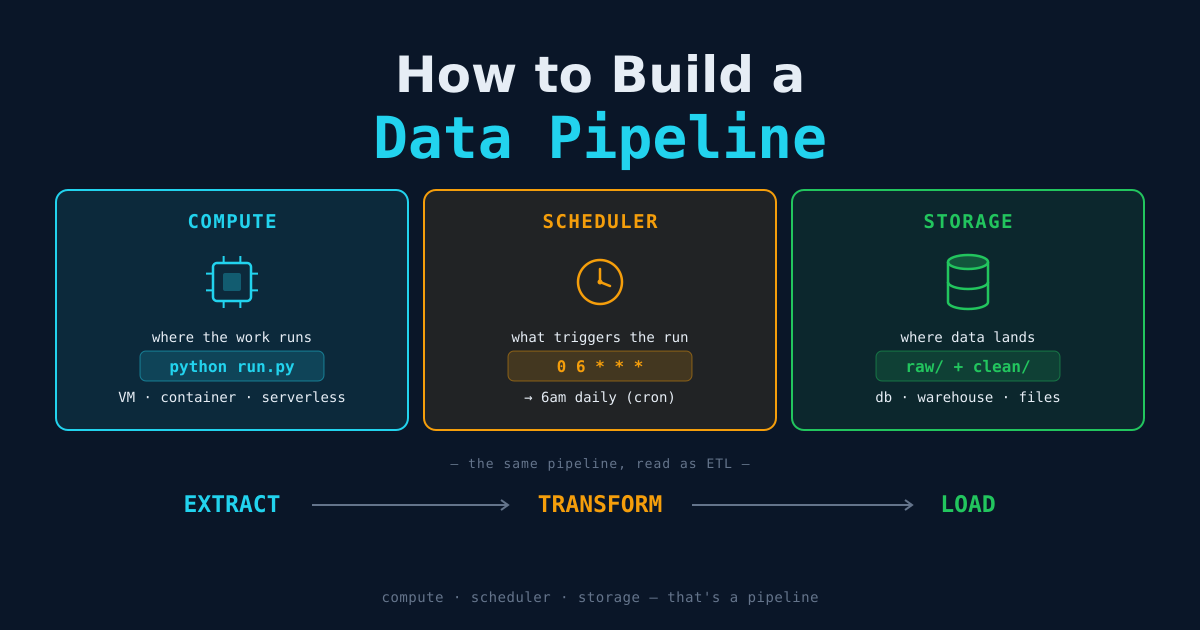
“Build a data pipeline” sounds like it requires a platform team and a budget. It doesn’t. Underneath the tooling, a pipeline is three decisions:
- Designated compute — where the work actually runs.
- A scheduler — what wakes the work up and triggers it.
- Storage — where the data lands and lives.
Get those three right and you have a pipeline. Everything else — orchestration tools, monitoring, retries, lineage — is refinement on top of these three pillars. This article walks through each one, and then shows that what you’ve built is just a textbook ETL wearing different clothes.
The Three Things Every Pipeline Needs
Before any code, picture the shape:
   ┌─────────────┐
   │  SCHEDULER  │  "run at 6am"
   └──────┬──────┘
          │ triggers
          ▼
   ┌─────────────┐
   │   COMPUTE   │  runs your code
   └──────┬──────┘
          │ writes to
          ▼
   ┌─────────────┐
   │   STORAGE   │  holds the result
   └─────────────┘
A scheduler decides when. Compute decides where the work happens. Storage decides where the output goes. If any one of the three is missing, you don’t have a pipeline — you have a script someone has to remember to run, or a result that vanishes when the process exits. Let’s take them one at a time.
1. Designated Compute
Compute is the machine — or process — that executes your pipeline code. The important word is designated: a known, repeatable place the work runs every time, not “wherever I happened to have a terminal open.”
The difference matters because a pipeline that only runs on your laptop has a single point of failure with a battery in it. The moment you close the lid, the pipeline stops. Designating compute means choosing a home for the work that doesn’t depend on you being awake.
Common choices, roughly from smallest to largest:
| Option | Good for | Trade-off |
|---|---|---|
| Your own laptop / desktop | First prototype, learning | Stops when the machine sleeps; not reproducible |
| A small always-on VM (EC2, Droplet) | Steady daily jobs | You patch and babysit the box |
| A container (Docker on a host, ECS, Cloud Run) | Reproducible dependencies | Need to build and store an image |
| A serverless function (Lambda, Cloud Functions, Workers) | Short, spiky jobs | Time and memory limits; cold starts |
| A managed worker (GitHub Actions runner, Airflow worker) | Jobs already near your CI or orchestrator | Tied to that platform’s quotas |
Three things make compute designated rather than incidental:
- It’s reproducible. The same Python version, the same installed packages, every run. A
requirements.txt(or a container image) pins this so the job doesn’t break the day your laptop upgrades a library. - It’s isolated from you. It runs whether or not you’re logged in. That’s the whole point of moving off the laptop.
- It’s sized for the job. A pipeline that loads ten thousand rows wants a tiny box. One that reshapes ten million rows in memory wants more RAM than a free tier gives you. Match the machine to the work, not to the logo on the invoice.
For a first real pipeline, a small always-on VM or a scheduled GitHub Actions runner is plenty. Don’t reach for a cluster to move a spreadsheet.
2. A Scheduler (Cron Is the Basic Example)
Compute runs the code, but something has to tell it to run. That’s the scheduler. The simplest, most universal scheduler — and the one worth learning first — is cron.
Cron is a daemon built into every Linux and macOS system. You give it a line with a time pattern and a command, and it runs that command on that schedule, forever, without you touching it again.
You edit your schedule with:
crontab -eAnd add a line like this to run a pipeline every day at 6:00 AM:
0 6 * * * /usr/bin/python3 /home/me/pipeline/run.py >> /home/me/pipeline/logs/run.log 2>&1That one line is a complete scheduler. Here’s how to read the five time fields in front of the command:
┌───────── minute        (0 - 59)
│ ┌─────── hour          (0 - 23)
│ │ ┌───── day of month  (1 - 31)
│ │ │ ┌─── month         (1 - 12)
│ │ │ │ ┌─ day of week   (0 - 6, Sunday = 0)
│ │ │ │ │
0 6 * * *   python3 run.py
An asterisk means “every.” So 0 6 * * * reads as minute 0, hour 6, every day, every month, every weekday — i.e. 6:00 AM daily. A few more patterns to anchor the syntax:
| Cron line | Meaning |
|---|---|
*/15 * * * * | Every 15 minutes |
0 * * * * | Top of every hour |
0 6 * * * | Every day at 6:00 AM |
0 6 * * 1 | Every Monday at 6:00 AM |
0 0 1 * * | Midnight on the 1st of each month |
Two details that trip people up on their first cron job:
- Cron has almost no environment. It doesn’t load your shell profile, so
$PATHis minimal and your virtualenv isn’t active. Use absolute paths (/usr/bin/python3, the full path torun.py) or activate the environment inside the command. - Redirect the output.
>> run.log 2>&1appends both normal output and errors to a log file. Without it, cron emails the output into a void you’ll never check, and a silent failure is the worst kind.
Cron is the basic example on purpose — it’s the floor, not the ceiling. When you outgrow it (you need retries, dependencies between jobs, backfills, or a dashboard of what ran), you graduate to an orchestrator like Airflow, Dagster, or Prefect. But they all do the same fundamental job cron does: decide when the compute runs. Learn cron first; the concepts transfer directly.
3. Storage
Compute produces data. Storage is where that data goes so it outlives the process that made it. A pipeline whose output only exists in memory, or in a file that gets overwritten and forgotten, hasn’t really moved data anywhere.
There’s no single right storage layer — there’s a right one for each stage of the data’s life:
| Storage type | Examples | Use it for |
|---|---|---|
| Object storage | S3, R2, GCS, a local data/raw/ folder | Raw, untouched source data — the landing zone |
| Relational database | PostgreSQL, SQLite, MySQL | Clean, queryable rows your apps and analysts hit |
| Data warehouse | Snowflake, BigQuery, DuckDB | Analytical queries over large, columnar tables |
| File formats | CSV, JSON, Parquet | Handoff between stages and tools |
The single most useful storage habit is to separate raw from processed:
data/
├── raw/        # exactly what the source gave you — never edited
└── clean/      # the transformed, validated output
Keeping a pristine copy of the raw data is what lets you re-run the rest of the pipeline without re-fetching from a rate-limited API. Your cleaning logic will change as you learn more about the data; when it does, you replay the transform against the raw files you already saved instead of going back to the source.
The other habit worth building in from day one is idempotency — running the pipeline twice should not double your data. Replacing a table wholesale, or upserting on a primary key, both achieve this. It’s the difference between a pipeline you can safely re-run after a failure and one that corrupts itself every time it hiccups.
Translating the Pipeline to an ETL
Here’s the reframe. You set up three things — compute, a scheduler, and storage — for practical reasons. But step back and look at what the data does as it flows through them, and you’ve built the most common pattern in data engineering: ETL — Extract, Transform, Load.
ETL describes the three things that happen to the data:
| ETL stage | What happens to the data |
|---|---|
| Extract | Pull it out of the source (an API, a file, another database) |
| Transform | Clean, reshape, deduplicate, and validate it |
| Load | Write it to its destination |
Now overlay that on the three pillars. They line up almost perfectly:
SCHEDULER  ──▶  COMPUTE  ──────────────────────▶  STORAGE
 (cron)         runs Extract→Transform→Load        raw + clean
                  │           │           │
              [Extract]  [Transform]    [Load]
                  │                       │
reads source writes result- The scheduler (your cron line) is what kicks off an ETL run.
- The compute is where Extract, Transform, and Load actually execute — it’s the engine the three ETL verbs run inside.
- The storage is both ends of ETL: Extract reads from a source and lands raw data in storage; Load writes the transformed result back to storage.
So the infrastructure question (“where does it run, what triggers it, where does the data go?”) and the data-flow question (“extract, transform, load”) are two views of the same pipeline. You built the plumbing; ETL is the name for the water moving through it.
A quick note on ELT — Extract, Load, Transform. Same three verbs, reordered: you load the raw data into a powerful warehouse first and transform it there with SQL, rather than transforming on your own compute before loading. The three pillars don’t change; you’re just choosing to do the “transform” work inside the storage layer’s compute instead of your own. Which order is right is its own decision — see the linked article below.
The Low Hanging Data Take
People stall on “build a data pipeline” because the phrase has accumulated a decade of heavyweight tooling around it. Strip that away and the assignment is small: pick a place for the work to run, give it a cron line so it runs without you, and choose where the data lands — keeping the raw copy separate from the clean one. That’s a pipeline. The moment it runs on a schedule and writes somewhere durable, you’ve done the thing.
The ETL vocabulary isn’t a fourth thing to build — it’s just the name for what your three pillars already do to the data. Build the plumbing first with the smallest tools that work (a VM, cron, a folder or a database), watch one real run go Extract → Transform → Load, and then reach for an orchestrator when cron genuinely starts to hurt. Start with the floor. The ceiling can wait.
Next Steps
- Building Your First Data Pipeline — The code-level companion to this article: actual
extract.py,transform.py, andload.pywired into a runnable pipeline. - Scheduling and Automating Data Pipelines — Going beyond a single cron line to retries, GitHub Actions, and orchestrators.
- ETL vs ELT: Choosing the Right Pipeline Pattern — When to transform before loading versus loading raw and transforming in the warehouse.