Contents
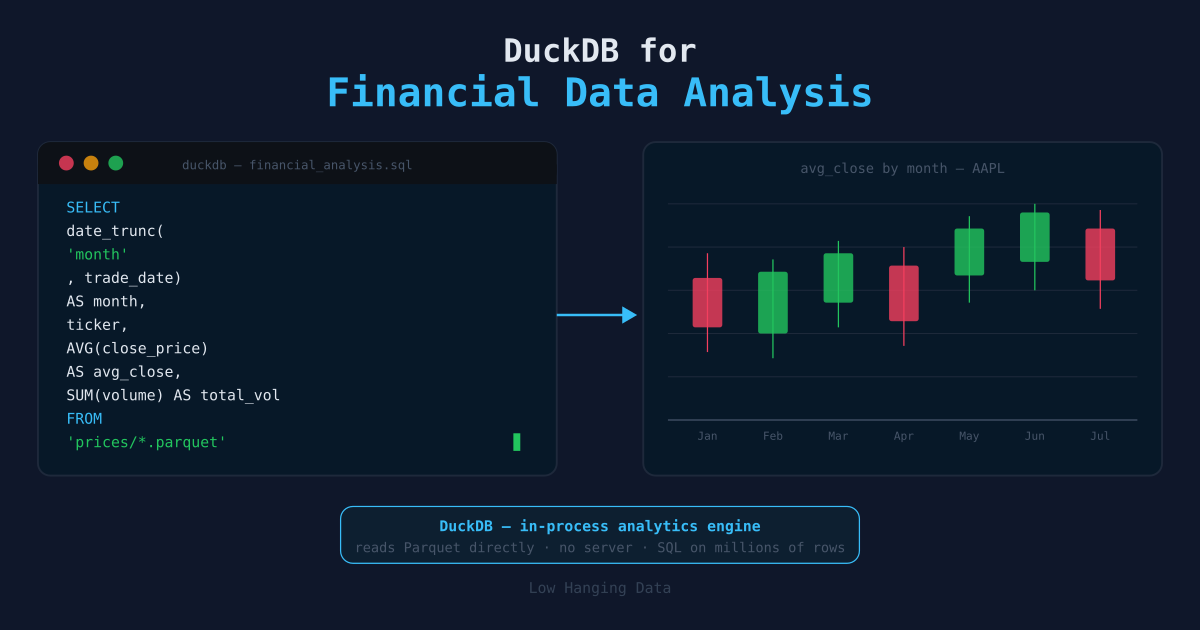
DuckDB for Financial Data Analysis
🌳 High Hanging Fruit
The Parquet and DuckDB article covers the basics: installing DuckDB, writing Parquet files, running queries. This article goes further — it uses stock market data as the working example and covers the patterns that come up repeatedly in financial analysis: rolling windows, returns, rank filtering, multi-file queries, and exporting results for downstream use.
Setting Up a Local Stock Data Store
Start with a directory of daily OHLCV CSV files — one per ticker, or one combined file. Convert to Parquet once and query many times.
import duckdb
from pathlib import Path

RAW = Path("data/raw")
PARQUET = Path("data/parquet")
PARQUET.mkdir(parents=True, exist_ok=True)

# Convert all CSVs to a single Parquet file, adding a ticker column
duckdb.sql(f"""
    COPY (
        SELECT
            filename_part AS ticker,
            CAST(Date AS DATE)      AS date,
            CAST(Open AS DOUBLE)    AS open,
            CAST(High AS DOUBLE)    AS high,
            CAST(Low AS DOUBLE)     AS low,
            CAST(Close AS DOUBLE)   AS close,
            CAST(Volume AS BIGINT)  AS volume
        FROM read_csv(
            '{RAW}/*.csv',
            filename_part = true,
            auto_detect = true
        )
    )
    TO '{PARQUET}/prices.parquet'
    (FORMAT PARQUET, COMPRESSION 'zstd')
""")
filename_part injects the source filename (without extension) as a column — a clean way to derive ticker from filename without pre-processing the CSVs.
OHLCV Data Quality Checks
Raw price data from free sources contains errors that are easy to miss and expensive to ignore. Run these checks immediately after ingestion, before any calculations.
import duckdb

issues = duckdb.sql("""
    SELECT
        ticker,
        date,
        open, high, low, close, volume,

        -- High must be >= all other prices
        CASE WHEN high < low                 THEN 'high < low'
             WHEN high < open                THEN 'high < open'
             WHEN high < close               THEN 'high < close'
             ELSE NULL END AS price_error,

        -- Zero or negative values are always wrong
        CASE WHEN close <= 0                 THEN 'non-positive close'
             WHEN volume < 0                 THEN 'negative volume'
             ELSE NULL END AS range_error,

        -- Price gaps larger than 50% in a single day suggest a split or bad data
        CASE WHEN ABS(
            close / NULLIF(LAG(close, 1) OVER (PARTITION BY ticker ORDER BY date), 0) - 1
        ) > 0.50 THEN 'large gap — possible split or bad tick'
             ELSE NULL END AS gap_warning

    FROM 'data/parquet/prices.parquet'
    WHERE price_error IS NOT NULL
       OR range_error IS NOT NULL
       OR gap_warning IS NOT NULL
    ORDER BY ticker, date
""").df()

if not issues.empty:
    print(f"Found {len(issues)} data quality issues:")
    print(issues.to_string())
Large single-day gaps are the most common surprise. They can mean:
- A stock split (adjust prices or use an adjusted-close data source)
- A missing trading day creating a phantom gap across a weekend or holiday
- A genuinely bad tick from the data provider
The right response depends on the cause — but you need to know the gap exists before you can decide.
A Note on Survivorship Bias
The tickers in your dataset are the ones that still exist. Companies that went bankrupt, were acquired, or were delisted during your study window are absent — but they were live trading candidates at the time. Training a model only on survivors inflates apparent returns because the worst outcomes are excluded by construction.
There is no simple fix from free data sources. Being aware of the bias is the first step: when your backtest shows strong performance, ask whether the result would hold for the full population of tradeable stocks at the time, not just the ones that survived to today.
Computing Returns
Daily and rolling returns are the foundation of almost every financial calculation.
import duckdb

result = duckdb.sql("""
    SELECT
        ticker,
        date,
        close,

        -- Daily return
        (close - LAG(close, 1) OVER w) / LAG(close, 1) OVER w AS daily_return,

        -- Cumulative return from first available date
        close / FIRST_VALUE(close) OVER w - 1 AS cum_return,

        -- Log return (for statistics)
        LN(close / LAG(close, 1) OVER w) AS log_return

    FROM 'data/parquet/prices.parquet'
    WINDOW w AS (PARTITION BY ticker ORDER BY date)
    ORDER BY ticker, date
""").df()
Using a named WINDOW clause avoids repeating the partition/order definition across every column.
Rolling Indicators
Simple and Exponential Moving Averages
DuckDB’s window functions handle rolling aggregations directly.
result = duckdb.sql("""
    SELECT
        ticker,
        date,
        close,

        -- 20-day simple moving average
        AVG(close) OVER (
            PARTITION BY ticker ORDER BY date
            ROWS BETWEEN 19 PRECEDING AND CURRENT ROW
        ) AS sma_20,

        -- 50-day SMA
        AVG(close) OVER (
            PARTITION BY ticker ORDER BY date
            ROWS BETWEEN 49 PRECEDING AND CURRENT ROW
        ) AS sma_50,

        -- 20-day rolling standard deviation (volatility proxy)
        STDDEV(close) OVER (
            PARTITION BY ticker ORDER BY date
            ROWS BETWEEN 19 PRECEDING AND CURRENT ROW
        ) AS vol_20

    FROM 'data/parquet/prices.parquet'
    ORDER BY ticker, date
""").df()
Relative Strength Index (RSI)
RSI requires computing average gains and losses, which maps cleanly onto window functions.
result = duckdb.sql("""
    WITH daily AS (
        SELECT
            ticker,
            date,
            close,
            close - LAG(close, 1) OVER (PARTITION BY ticker ORDER BY date) AS chg
        FROM 'data/parquet/prices.parquet'
    ),
    gains_losses AS (
        SELECT
            ticker,
            date,
            close,
            GREATEST(chg, 0) AS gain,
            ABS(LEAST(chg, 0)) AS loss
        FROM daily
        WHERE chg IS NOT NULL
    )
    SELECT
        ticker,
        date,
        close,
        100 - (100 / (1 + (
            AVG(gain) OVER (
                PARTITION BY ticker ORDER BY date
                ROWS BETWEEN 13 PRECEDING AND CURRENT ROW
            ) /
            NULLIF(AVG(loss) OVER (
                PARTITION BY ticker ORDER BY date
                ROWS BETWEEN 13 PRECEDING AND CURRENT ROW
            ), 0)
        ))) AS rsi_14
    FROM gains_losses
    ORDER BY ticker, date
""").df()
Querying Multiple Tickers at Once
DuckDB’s IN operator and WHERE filtering push efficiently into Parquet column statistics.
WATCHLIST = ["AAPL", "MSFT", "NVDA", "GOOGL", "AMZN"]

result = duckdb.sql(f"""
    SELECT *
    FROM 'data/parquet/prices.parquet'
    WHERE ticker IN ({', '.join(f"'{t}'" for t in WATCHLIST)})
      AND date >= '2024-01-01'
    ORDER BY ticker, date
""").df()
For larger watchlists, pass a list directly using DuckDB’s Python parameter binding:
import duckdb

con = duckdb.connect()
con.execute("CREATE TABLE watchlist AS SELECT unnest(?) AS ticker", [WATCHLIST])

result = con.execute("""
    SELECT p.*
    FROM 'data/parquet/prices.parquet' p
    JOIN watchlist w ON p.ticker = w.ticker
    WHERE p.date >= '2024-01-01'
""").df()
Ranking and Filtering
Find the top performers by return over a rolling window — a common screening task.
result = duckdb.sql("""
    WITH returns AS (
        SELECT
            ticker,
            date,
            close / NULLIF(LAG(close, 20) OVER (
                PARTITION BY ticker ORDER BY date
            ), 0) - 1 AS ret_20d
        FROM 'data/parquet/prices.parquet'
    )
    SELECT *
    FROM (
        SELECT
            ticker,
            date,
            ret_20d,
            RANK() OVER (PARTITION BY date ORDER BY ret_20d DESC) AS rank_desc
        FROM returns
        WHERE ret_20d IS NOT NULL
    )
    WHERE rank_desc <= 5
    ORDER BY date DESC, rank_desc
""").df()
This returns the top 5 tickers by 20-day return for each trading day — a momentum screen.
Joining Prices with External Signals
The stock sentiment pipeline produces a CSV of sentiment scores by ticker and date. Join it directly against the price Parquet without materializing either dataset.
result = duckdb.sql("""
    SELECT
        p.ticker,
        p.date,
        p.close,
        (p.close - LAG(p.close, 1) OVER (PARTITION BY p.ticker ORDER BY p.date))
            / LAG(p.close, 1) OVER (PARTITION BY p.ticker ORDER BY p.date) AS ret_1d,
        s.reddit_sentiment,
        s.google_trends_score,
        s.headline_sentiment
    FROM 'data/parquet/prices.parquet' p
    LEFT JOIN read_csv_auto('data/signals/sentiment.csv') s
        ON p.ticker = s.ticker AND p.date = CAST(s.date AS DATE)
    WHERE p.date >= '2023-01-01'
    ORDER BY p.ticker, p.date
""").df()
DuckDB handles the join between a Parquet file and a CSV in a single query — no staging tables needed.
Persisting Results
For long-running queries you run repeatedly, write results back to Parquet.
duckdb.sql("""
    COPY (
        SELECT
            ticker,
            date,
            close,
            AVG(close) OVER (
                PARTITION BY ticker ORDER BY date
                ROWS BETWEEN 19 PRECEDING AND CURRENT ROW
            ) AS sma_20,
            AVG(close) OVER (
                PARTITION BY ticker ORDER BY date
                ROWS BETWEEN 49 PRECEDING AND CURRENT ROW
            ) AS sma_50,
            STDDEV(close) OVER (
                PARTITION BY ticker ORDER BY date
                ROWS BETWEEN 19 PRECEDING AND CURRENT ROW
            ) AS vol_20
        FROM 'data/parquet/prices.parquet'
        ORDER BY ticker, date
    )
    TO 'data/parquet/prices_with_indicators.parquet'
    (FORMAT PARQUET, COMPRESSION 'zstd')
""")
Subsequent queries read the pre-computed indicators instead of recomputing them on every run.
Exporting for Machine Learning
The final feature matrix for model training is usually a flat DataFrame. DuckDB can produce it in one query.
import duckdb
import pandas as pd

features = duckdb.sql("""
    SELECT
        ticker,
        date,
        -- Price features
        close,
        (close - LAG(close, 1) OVER w) / LAG(close, 1) OVER w AS ret_1d,
        (close - LAG(close, 5) OVER w) / LAG(close, 5) OVER w AS ret_5d,
        AVG(close) OVER (PARTITION BY ticker ORDER BY date ROWS BETWEEN 19 PRECEDING AND CURRENT ROW) / close - 1 AS dist_sma20,

        -- Sentiment features (from joined CSV)
        s.reddit_sentiment,
        s.google_trends_score,

        -- Target: next-day return direction
        SIGN(
            (LEAD(close, 1) OVER w - close) / close
        ) AS target

    FROM 'data/parquet/prices.parquet' p
    LEFT JOIN read_csv_auto('data/signals/sentiment.csv') s
        ON p.ticker = s.ticker AND p.date = CAST(s.date AS DATE)
    WINDOW w AS (PARTITION BY ticker ORDER BY date)
    ORDER BY ticker, date
""").df()

# Drop rows where any feature or target is null
features = features.dropna()
This pattern — build the full feature matrix in SQL, hand off a clean DataFrame to sklearn — keeps the data transformation logic in one place and makes it reproducible.
Performance Tips
- Filter early. Put date and ticker filters in the query, not after
.df(). DuckDB pushes filters into Parquet file statistics. - Use persistent connections for repeated queries.
duckdb.connect("analytics.duckdb")creates a persistent database file. Register Parquet views once, query them many times. - Parallelism is automatic. DuckDB uses all available CPU cores by default. No configuration needed.
Next Steps
- Working with Parquet and DuckDB — Setup, file writes, and basic queries.
- Low-Hanging Data Sources for Stock Prediction — What signals to add to the feature matrix built above.
- Building Your First Data Pipeline — Wrapping these queries in a reproducible pipeline.