Contents

Data wrangling is the work of transforming raw data into a clean, consistent shape. Raw data from APIs, exports, and file dumps almost always needs cleaning before it’s useful — missing values, wrong types, inconsistent formatting, duplicate rows. Pandas is the standard Python tool for this work.

Loading Data into a DataFrame

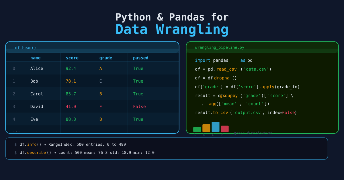
A DataFrame is a table — rows and columns, like a spreadsheet or database table — held in memory.

import pandas as pd

# From a CSV file
df = pd.read_csv("data/raw/users.csv")

# From a JSON file
df = pd.read_json("data/raw/events.json")

# From a list of dicts (e.g. API response)
records = [
    {"id": 1, "name": "Alice", "score": 92},
    {"id": 2, "name": "Bob",   "score": None},
]
df = pd.DataFrame(records)

Understanding Your Data

Before cleaning, look at what you have:

df.shape          # (rows, columns)
df.dtypes         # column data types
df.head(10)       # first 10 rows
df.tail(5)        # last 5 rows
df.info()         # summary: types, non-null counts
df.describe()     # stats for numeric columns
df.isnull().sum() # count of missing values per column
df.duplicated().sum()  # count of duplicate rows

Selecting and Filtering

# Select a single column (returns a Series)
df["name"]

# Select multiple columns (returns a DataFrame)
df[["name", "email", "score"]]

# Filter rows by condition
df[df["score"] > 80]
df[df["city"] == "Chicago"]

# Multiple conditions (use & and | with parentheses)
df[(df["score"] > 70) & (df["active"] == True)]
df[(df["city"] == "Austin") | (df["city"] == "Dallas")]

# Filter with .query() — often more readable
df.query("score > 70 and active == True")

Handling Missing Values

The most important thing to know about missing values is that there’s no universal right answer — the correct strategy depends on why the data is missing. Dropping nulls is the easiest choice and often the wrong one. If 30% of your rows have a null in one column, dropping them doesn’t clean your data; it removes 30% of your signal.

# Drop rows where any column is null
df.dropna()

# Drop rows where a specific column is null
df.dropna(subset=["email"])

# Fill nulls with a fixed value
df["score"].fillna(0)
df["city"].fillna("Unknown")

# Fill nulls with the column mean
df["score"].fillna(df["score"].mean())

# Forward-fill (useful for time series)
df["value"].ffill()

Always think before dropping rows. If 40% of your data has a null email, dropping those rows may destroy your dataset. Consider whether the null means “no email” (fill with empty string) or “bad data” (investigate).

Fixing Data Types

Pandas sometimes infers the wrong type, especially from CSV files:

# Inspect types
print(df.dtypes)

# Convert a column to a specific type
df["age"] = df["age"].astype(int)
df["score"] = df["score"].astype(float)
df["user_id"] = df["user_id"].astype(str)

# Parse dates (very common)
df["created_at"] = pd.to_datetime(df["created_at"])

# Handle date parsing errors gracefully
df["created_at"] = pd.to_datetime(df["created_at"], errors="coerce")
# invalid dates become NaT (Not a Time) instead of raising an exception

Renaming and Reordering Columns

# Rename specific columns
df = df.rename(columns={
    "user_id": "id",
    "full_name": "name",
    "signup_date": "created_at",
})

# Rename all columns to lowercase with underscores
df.columns = df.columns.str.lower().str.replace(" ", "_")

# Select and reorder columns
df = df[["id", "name", "email", "created_at", "score"]]

Cleaning String Data

String operations in pandas use the .str accessor:

# Remove leading/trailing whitespace
df["name"] = df["name"].str.strip()

# Normalize case
df["email"] = df["email"].str.lower()
df["city"]  = df["city"].str.title()

# Extract part of a string
df["domain"] = df["email"].str.split("@").str[1]

# Replace values
df["status"] = df["status"].str.replace("cancelled", "canceled")

# Check for pattern
df["is_gmail"] = df["email"].str.endswith("@gmail.com")

Deduplication

# Drop exact duplicate rows
df = df.drop_duplicates()

# Drop duplicates based on specific columns (keep first occurrence)
df = df.drop_duplicates(subset=["email"], keep="first")

# Drop duplicates, keep the most recent (sort first)
df = df.sort_values("created_at", ascending=False)
df = df.drop_duplicates(subset=["email"], keep="first")

Adding and Transforming Columns

# Add a new column
df["full_name"] = df["first_name"] + " " + df["last_name"]

# Apply a function to each row
df["score_grade"] = df["score"].apply(lambda x: "pass" if x >= 60 else "fail")

# Apply a function row-wise (multiple columns)
def categorize(row):
    if row["score"] >= 90:
        return "A"
    elif row["score"] >= 80:
        return "B"
    else:
        return "C"

df["grade"] = df.apply(categorize, axis=1)

.apply() with a Python function is the most expensive operation in pandas. It iterates row by row under the hood, bypassing the vectorized C code that makes pandas fast. Before reaching for .apply(), check whether there’s a vectorized alternative: .str methods, arithmetic on the whole column, or np.where(). On a million rows, the difference between .apply() and a vectorized operation can be 100x.

# Map values to new values
status_map = {"active": 1, "inactive": 0, "pending": 0}
df["is_active"] = df["status"].map(status_map)

Grouping and Aggregating

# Count by group
df.groupby("city")["id"].count()

# Multiple aggregations
df.groupby("city").agg(
    user_count=("id", "count"),
    avg_score=("score", "mean"),
    total_score=("score", "sum"),
)

# Reset index so the result is a clean DataFrame
summary = df.groupby("status")["amount"].sum().reset_index()
summary.columns = ["status", "total_amount"]

Merging DataFrames

The pandas equivalent of a SQL JOIN — with one trap that catches almost everyone at least once: if both DataFrames have duplicate keys, pd.merge() produces a cartesian product of every matching pair. Three rows with user_id=1 on the left and four rows with user_id=1 on the right gives you twelve rows in the output — silently, with no warning. Always check len(df) before and after a merge until you’re certain the keys are clean.

users = pd.read_csv("users.csv")
orders = pd.read_csv("orders.csv")

# Inner join (only matching rows)
merged = pd.merge(orders, users, on="user_id", how="inner")

# Left join (all orders, with user info where available)
merged = pd.merge(orders, users, on="user_id", how="left")

# Join on columns with different names
merged = pd.merge(
    orders, users,
    left_on="customer_id",
    right_on="id",
    how="left"
)

Saving Clean Data

# Save to CSV
df.to_csv("data/clean/users.csv", index=False)

# Save to JSON
df.to_json("data/clean/users.json", orient="records", indent=2)

# Save to SQLite
import sqlite3
conn = sqlite3.connect("data/journal.db")
df.to_sql("users", conn, if_exists="replace", index=False)
conn.close()

# Save to Parquet (efficient for large files)
df.to_parquet("data/clean/users.parquet")

A Minimal Cleaning Pipeline

import pandas as pd

def clean_users(raw_path, clean_path):
    df = pd.read_csv(raw_path)

    # Normalize column names
    df.columns = df.columns.str.lower().str.replace(" ", "_")

    # Drop rows without a valid email
    df = df.dropna(subset=["email"])

    # Normalize strings
    df["email"] = df["email"].str.strip().str.lower()
    df["name"]  = df["name"].str.strip().str.title()

    # Parse dates
    df["created_at"] = pd.to_datetime(df["created_at"], errors="coerce")

    # Deduplicate
    df = df.drop_duplicates(subset=["email"], keep="first")

    # Save
    df.to_csv(clean_path, index=False)
    print(f"Cleaned {len(df)} records → {clean_path}")

clean_users("data/raw/users.csv", "data/clean/users.csv")

Memory Usage and When to Switch Tools

Pandas holds the entire DataFrame in memory. For typical data work — files under a few hundred megabytes — this is fine. At larger sizes, it becomes the bottleneck.

Checking Memory Usage

# Total memory used by the DataFrame
print(df.memory_usage(deep=True).sum() / 1_024**2, "MB")

# Per-column breakdown
print(df.memory_usage(deep=True).sort_values(ascending=False))

deep=True counts the actual size of string data, not just pointers. Without it, object columns appear much smaller than they are.

Reducing Memory with Downcasting

Many DataFrames use more memory than necessary because pandas defaults to 64-bit types:

# Downcast integers (int64 → smallest int that fits the values)
df["age"]    = pd.to_numeric(df["age"],    downcast="integer")
df["count"]  = pd.to_numeric(df["count"],  downcast="integer")

# Downcast floats (float64 → float32 where precision is not critical)
df["price"]  = pd.to_numeric(df["price"],  downcast="float")

# Convert low-cardinality string columns to categoricals
# Useful when a column has few unique values (status, city, category)
df["status"] = df["status"].astype("category")

Categorical encoding is especially effective on columns like ticker (10 unique values across 1 million rows): it stores an integer lookup table instead of repeating the string on every row.

When Pandas Is the Wrong Tool

Situation	Better tool
File is too large to fit in RAM	DuckDB (query in chunks) or Polars (lazy evaluation)
Need fast column operations on 10M+ rows	Polars (pip install polars)
Need distributed processing across machines	Dask or Spark
All you need is SQL aggregations on a file	duckdb.sql("SELECT ... FROM 'file.parquet'") — skip pandas entirely

A rough rule: if df.memory_usage(deep=True).sum() exceeds half your available RAM, or if your transformations take more than a minute on a modern laptop, evaluate DuckDB or Polars first. Both support a pandas-compatible API and are significantly faster on large datasets.

Next Steps

• Building Your First Data Pipeline — Combine collection, cleaning, and storage into an automated workflow.
• Organizing Data with SQL — Query your clean data with SQL.
• Data Cleaning and Validation — Systematic techniques for handling missing values, duplicates, and type mismatches.