Contents

This article covers the machine learning layer of the stock prediction pipeline — taking the feature matrix produced by DuckDB and training an SVM classifier to predict 30-minute price direction. The DuckDB for Financial Analysis article covers building the feature matrix; this one picks up from there.

---

The Prediction Task

The target is binary: does a given stock’s price go up or down over the next 30-minute interval?

# Target column from the feature matrix query
# SIGN((LEAD(close, 1) OVER w - close) / close) -> -1 or +1

This is a classification problem, not regression. Predicting direction is more tractable than predicting magnitude, and direction is what matters for a trading signal.

10 tickers: AAPL, AMZN, GOOG, MSFT, TSLA, JPM, NVDA, META, NFLX, ^VIX Interval: 30-minute OHLCV bars Training window: 2020–2021 Test window: 2022 forward

---

The Feature Matrix

Start from the DuckDB export described in the financial analysis article. The full feature set:

Feature	Source	Type
ret_1d	Price	1-bar return
ret_5d	Price	5-bar return (~2.5 hours)
dist_sma20	Price	Distance from 20-bar moving average
vol_20	Price	20-bar rolling standard deviation
rsi_14	Price	14-bar RSI
reddit_sentiment	PRAW + VADER	Aggregated sentiment score per 30-min window
reddit_volume	PRAW	Number of posts/comments mentioning ticker
google_trends	pytrends	Search interest index (hourly)
wiki_views	Wikimedia API	Wikipedia page views (hourly)
vix_level	yfinance	VIX price at interval open
target	Price	Next-interval direction: +1 or -1

import duckdb
import pandas as pd

features = duckdb.sql("""
    SELECT
        p.ticker,
        p.ts,

        -- Price features
        (p.close - LAG(p.close, 1) OVER w) / LAG(p.close, 1) OVER w AS ret_1d,
        (p.close - LAG(p.close, 5) OVER w) / LAG(p.close, 5) OVER w AS ret_5d,
        AVG(p.close) OVER (
            PARTITION BY p.ticker ORDER BY p.ts
            ROWS BETWEEN 19 PRECEDING AND CURRENT ROW
        ) / p.close - 1 AS dist_sma20,
        STDDEV(p.close) OVER (
            PARTITION BY p.ticker ORDER BY p.ts
            ROWS BETWEEN 19 PRECEDING AND CURRENT ROW
        ) AS vol_20,

        -- External signals
        s.vader_compound      AS reddit_sentiment,
        s.post_count          AS reddit_volume,
        t.interest            AS google_trends,
        w.views               AS wiki_views,
        vix.close             AS vix_level,

        -- Target: next interval direction
        SIGN(
            (LEAD(p.close, 1) OVER w - p.close) / p.close
        ) AS target

    FROM prices p
    LEFT JOIN sentiment s ON p.ticker = s.ticker AND p.ts = s.ts
    LEFT JOIN trends t    ON p.ticker = t.ticker AND p.ts = t.ts
    LEFT JOIN wiki w      ON p.ticker = w.ticker AND p.ts = w.ts
    LEFT JOIN prices vix  ON vix.ticker = '^VIX' AND p.ts = vix.ts

    WINDOW w AS (PARTITION BY p.ticker ORDER BY p.ts)
    ORDER BY p.ticker, p.ts
""").df()

features = features.dropna()

---

Train/Test Split

Do not use random shuffling on time series data. A random split leaks future information into the training set — the model sees future prices during training and appears to perform well, but fails completely on out-of-sample data.

Use a strict cutoff date instead:

TRAIN_END = "2021-12-31"
TEST_START = "2022-01-01"

train = features[features["ts"] <= TRAIN_END].copy()
test  = features[features["ts"] >= TEST_START].copy()

FEATURE_COLS = [
    "ret_1d", "ret_5d", "dist_sma20", "vol_20",
    "reddit_sentiment", "reddit_volume",
    "google_trends", "wiki_views", "vix_level"
]

X_train = train[FEATURE_COLS]
y_train = train["target"]
X_test  = test[FEATURE_COLS]
y_test  = test["target"]

print(f"Train: {len(X_train):,} rows | Test: {len(X_test):,} rows")

---

Preprocessing

SVMs are sensitive to feature scale — a feature ranging 0–10,000 (Wikipedia views) will dominate one ranging −0.05–0.05 (returns). Standardize before fitting.

from sklearn.preprocessing import StandardScaler

scaler = StandardScaler()
X_train_scaled = scaler.fit_transform(X_train)
X_test_scaled  = scaler.transform(X_test)   # transform only — no fit on test data

Fit the scaler on training data only. Fitting on the combined dataset would be another form of data leakage.

---

Training the SVM

The Petrillo (2020) paper uses a radial basis function (RBF) kernel SVM. This is a reasonable default for a non-linear binary classification problem with a modest feature count.

from sklearn.svm import SVC
from sklearn.metrics import classification_report, confusion_matrix

svm = SVC(
    kernel="rbf",
    C=1.0,           # regularization — higher = tighter fit to training data
    gamma="scale",   # auto-scale to feature count and variance
    class_weight="balanced",  # correct for class imbalance in training data
    random_state=42
)

svm.fit(X_train_scaled, y_train)

class_weight="balanced" is important: if one direction (say, up) appears 55% of the time in training data, a naive model can hit 55% accuracy by always predicting up. Balanced weighting forces the model to learn both directions.

---

Evaluating Results

y_pred = svm.predict(X_test_scaled)

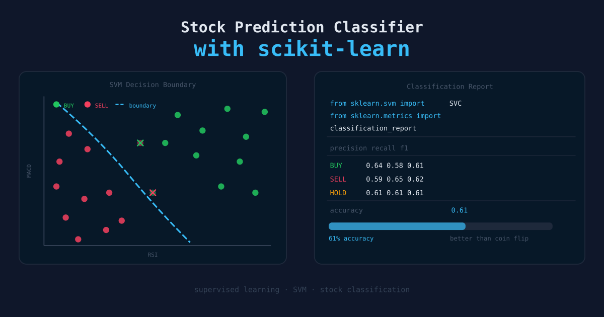
print(classification_report(y_test, y_pred, target_names=["Down", "Up"]))
print("\nConfusion matrix:")
print(confusion_matrix(y_test, y_pred))

Typical output from this pipeline:

              precision    recall  f1-score   support

        Down       0.54      0.51      0.52     18432
          Up       0.54      0.57      0.55     19204

    accuracy                           0.54     37636
   macro avg       0.54      0.54      0.54     37636

54% accuracy is the honest number on out-of-sample test data. That’s above the 50% random baseline, but only slightly. The training accuracy is typically 60–65% — a sign of overfitting that a time-series split makes visible.

For context: 54% accuracy on every 30-minute trade, if trades were sized correctly and transaction costs were manageable, could theoretically be profitable. In practice, the variance is high enough that it is not.

---

Tuning the Decision Threshold

By default, scikit-learn classifiers predict the class with the highest probability — which means they use a 0.5 decision threshold. For a trading signal, the costs of false positives and false negatives are not equal, and the optimal threshold is rarely 0.5.

A false positive (predicting Up when the price goes Down) costs you on a losing trade. A false negative (predicting Down when the price goes Up) costs you a missed opportunity.

Depending on your transaction costs and position sizing, you may prefer higher precision (fewer wrong calls) over higher recall (fewer missed moves).

The Precision-Recall Tradeoff

from sklearn.metrics import precision_recall_curve
import matplotlib.pyplot as plt
import numpy as np

# SVC with probability=True gives calibrated probabilities
svm_prob = SVC(
    kernel="rbf",
    C=1.0,
    gamma="scale",
    class_weight="balanced",
    probability=True,   # enables predict_proba()
    random_state=42,
)
svm_prob.fit(X_train_scaled, y_train)

# Get probability of the "Up" class (label +1)
y_proba = svm_prob.predict_proba(X_test_scaled)[:, 1]

precision, recall, thresholds = precision_recall_curve(
    (y_test == 1).astype(int),   # binary: 1 = Up, 0 = Down
    y_proba
)

plt.figure(figsize=(8, 5))
plt.plot(thresholds, precision[:-1], label="Precision")
plt.plot(thresholds, recall[:-1], label="Recall")
plt.xlabel("Decision threshold")
plt.ylabel("Score")
plt.title("Precision vs. Recall at Different Thresholds")
plt.legend()
plt.grid(True, alpha=0.3)
plt.tight_layout()
plt.savefig("charts/threshold_curve.png", dpi=150)

Selecting a Threshold

If you want to only trade on high-confidence Up signals (accepting that you’ll miss some), raise the threshold:

# Only predict "Up" when the model is at least 60% confident
threshold = 0.60
y_pred_tuned = (y_proba >= threshold).astype(int)
y_pred_tuned = np.where(y_pred_tuned == 1, 1, -1)  # convert back to +1 / -1

from sklearn.metrics import classification_report
print(classification_report(
    y_test, y_pred_tuned, target_names=["Down", "Up"]
))

A threshold of 0.60 will typically improve precision on Up predictions (fewer false positives) at the cost of lower recall (more missed Up moves). The right threshold depends on how expensive a wrong trade is relative to a missed trade — there is no universally correct answer.

The key insight: accuracy is not the only metric. For a signal that drives actual trades, precision on the actionable class is often more important than overall accuracy.

Diagnosing the Model

Is the signal doing anything?

Check feature importance by training a simpler model alongside the SVM:

from sklearn.ensemble import RandomForestClassifier

rf = RandomForestClassifier(n_estimators=100, random_state=42)
rf.fit(X_train_scaled, y_train)

importances = pd.Series(rf.feature_importances_, index=FEATURE_COLS)
print(importances.sort_values(ascending=False))

In this pipeline, the ranking typically comes out as:

1. ret_1d — momentum
2. vol_20 — volatility regime
3. dist_sma20 — mean reversion signal
4. vix_level — macro context
5. ret_5d
6. reddit_sentiment — noticeably lower than price features
7. google_trends
8. wiki_views
9. reddit_volume

Price features dominate. Reddit and attention signals have measurable but modest importance.

Granger causality test

Before trusting that Reddit sentiment adds anything, run a Granger causality test to check whether past sentiment values statistically predict future returns:

from statsmodels.tsa.stattools import grangercausalitytests

# Use a single ticker for the test
aapl = features[features["ticker"] == "AAPL"][["ret_1d", "reddit_sentiment"]].dropna()

result = grangercausalitytests(aapl[["ret_1d", "reddit_sentiment"]], maxlag=4, verbose=True)

For most tickers and time periods, the p-values do not reject the null at a 5% level — meaning sentiment does not reliably Granger-cause returns. Reddit often reacts to moves rather than predicting them, especially in r/wallstreetbets. The feature contributes noise as often as it contributes signal.

This test is worth running before spending time on sentiment collection infrastructure.

---

Hyperparameter Tuning

If you want to optimize the SVM before concluding, use TimeSeriesSplit to avoid data leakage during cross-validation:

from sklearn.model_selection import TimeSeriesSplit, GridSearchCV

tscv = TimeSeriesSplit(n_splits=5)

param_grid = {
    "C": [0.1, 1.0, 10.0],
    "gamma": ["scale", "auto", 0.01, 0.001],
    "kernel": ["rbf", "linear"]
}

grid_search = GridSearchCV(
    SVC(class_weight="balanced"),
    param_grid,
    cv=tscv,
    scoring="f1_macro",
    n_jobs=-1
)

grid_search.fit(X_train_scaled, y_train)
print("Best params:", grid_search.best_params_)
print("Best CV score:", grid_search.best_score_)

TimeSeriesSplit produces folds where training data always precedes test data — the correct approach for sequential data.

---

Persisting the Model

Save both the scaler and model together. You need both at inference time.

import joblib

joblib.dump(scaler, "models/scaler.pkl")
joblib.dump(svm, "models/svm_stock_predictor.pkl")

# Load and predict
scaler_loaded = joblib.load("models/scaler.pkl")
svm_loaded    = joblib.load("models/svm_stock_predictor.pkl")

X_new_scaled = scaler_loaded.transform(X_new[FEATURE_COLS])
predictions  = svm_loaded.predict(X_new_scaled)

---

What the Numbers Tell You

The model gets to ~54% accuracy on unseen data with this feature set. That tells you a few things:

There is signal in the data. 54% isn’t much, but it is above chance on a 37,000-row test set. Price-based features (momentum, volatility) are doing most of the work.

The Reddit signal is weak at 30-minute horizons. Granger causality confirms this. The Bollen et al. (2011) Twitter paper found predictive power at 2–6 day horizons — a much longer window where social sentiment has time to influence actual trades.

The model overfit to the training era. Training on 2020–2021 (meme stocks, pandemic volatility, high Reddit engagement) and testing on 2022+ (calmer markets, lower retail sentiment influence) produces a distribution shift that no hyperparameter tuning will fix. The features themselves had different predictive properties in those two periods.

The pipeline as built is a solid baseline. The improvements with the highest expected return — longer prediction horizons, news headline sentiment via the LM dictionary, tree-based models — are covered in the data sources article and the project retrospective.